
バックナンバーはこちら。
https://www.simulationroom999.com/blog/compare-matlabpythonscilabjulia-backnumber/
はじめに
前回は、MATLABによるDCモータ状態空間モデルのシミュレーションを実施。
今回は、これのPython(Numpy)版
登場人物
博識フクロウのフクさん

イラストACにて公開の「kino_k」さんのイラストを使用しています。
https://www.ac-illust.com/main/profile.php?id=iKciwKA9&area=1
エンジニア歴8年の太郎くん

イラストACにて公開の「しのみ」さんのイラストを使用しています。
https://www.ac-illust.com/main/profile.php?id=uCKphAW2&area=1
【再掲】DCモータ状態空間モデル
まずはDCモータ状態空間モデルを再掲しておこう。
状態方程式
\(
\begin{bmatrix}
\dot{\theta}(t) \\
\dot{\omega}(t) \\
\dot{I}(t)
\end{bmatrix}=
\begin{bmatrix}
0 && 1 && 0 \\
0 && 0 && K/J \\
0 && -K/L && -R/L
\end{bmatrix}
\begin{bmatrix}
\theta(t) \\
\omega(t) \\
I(t)
\end{bmatrix}+
\begin{bmatrix}
0 \\
0 \\
1/L
\end{bmatrix}
E(t)
\)
出力方程式
\(
\boldsymbol{y}=
\begin{bmatrix}
1 && 0 && 0 \\
0 && 1 && 0 \\
0 && 0 && 1 \\
\end{bmatrix}
\begin{bmatrix}
\theta(t) \\
\omega(t) \\
I(t)
\end{bmatrix}+
\begin{bmatrix}
0 \\
0 \\
0
\end{bmatrix}
E(t)
\)
今回はこれをPython(Numpy)で実現するんだね。
Pythonコード
そしてPythonコードは以下となる。
import numpy as np
import matplotlib.pyplot as plt

def statespacemodel(A,B,C,D,u,dt,x):
  # 状態方程式
  x = x + (A@x + B@u) * dt

  # 出力方程式
  y = C@x + D@u
  return x,y

def statespacemodel_motor():
  K=0.016
  J=0.000000919
  R=1.34
  L=0.00012

  A=np.array([[0,1,0],[0,0,K/J],[0,-K/L,-R/L]])
  B=np.array([[0],[0],[1/L]])
  C=np.array([[1,0,0],[0,1,0],[0,0,1]])
  D=np.array([[0],[0],[0]])

  dt = 0.0001
  t = np.linspace(0, 10, 100000) # 時間(横)軸
  u = np.zeros((1,100000))	# 入力信号生成
  u[0][50000:100000]=1	# 5秒後に0から1へ
  y = np.zeros((3,len(t)))
  x = np.zeros((3,1))

  for i in range(0, len(t)):
    x,y[:,[i]] = statespacemodel(A,B,C,D,u[:,[i]],dt,x)

  fig = plt.figure()
  ax1 = fig.add_subplot(3, 1, 1)
  ax2 = fig.add_subplot(3, 1, 2)
  ax3 = fig.add_subplot(3, 1, 3)

  ax1.plot(t,u.T)
  ax1.set_xlim(4.95,5.25)
  ax2.plot(t,y[0:2,:].T)
  ax2.set_xlim(4.95,5.25)
  ax2.set_ylim(-1,80)
  ax3.plot(t,y[2,:].T)
  ax3.set_xlim(4.95,5.25)

  plt.show()

if __name__ == "__main__":
statespacemodel_motor()流れとしてはMATLABと一緒だね。
あと、状態空間モデルの演算部分が変わってない点も一緒。
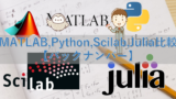
シミュレーション
そしてシミュレーション結果
MATLABでやったときと同じ結果が得られてるからOKってところか。
まとめ
まとめだよ。
- DCモータ状態空間モデルをPython(Numpy)でシミュレーション。
- 流れとしてはMATLABと一緒。
- 状態空間モデルの演算用関数が変化しない特徴も一緒。
- シミュレーションも同一であり、想定通り。
バックナンバーはこちら。

コメント